Construction Derby: Structured Data Generation with JSON Mode

Author's Note

This article was written prior to the public availability of Structured Outputs in OpenAI and was originally scheduled for release on the day of the announcement. The information remains relevant for open source models, but there is more to consider now with OpenAI's offering.

Introduction

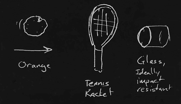
When making orange juice one can choose from a fair variety of extraction methods. Each option has differences in yield, quality of output, effort required, and failure modes, among other things. Deconstructing an orange into its constituent particles represents a significant investment of effort and a substantial likelihood of a sternly worded letter from the local nuclear regulatory agency¹, but yields an arguably pure product. Placing an untouched orange in a glass is arguably the minimal amount of effort but leads to a number of philosophical questions about the definition of orange juice. This could be considered “full pulp”. Nearly all of engineering is choosing between tradeoffs. Picking structured data generation options is no exception.

When it comes to generating JSON from unstructured text input, there are three major candidates: function calling, json mode, and prompt MacGyvering. We’ll go into detail about what each of these is, the latency overhead of using them, the benefits they offer, the problems they have, and ultimately how one should structure their code to make best use of the vast number of tools for automatically untangling the messy web of reality.

A Note on Evaluation

It's not a secret that natural language is messy, and being able to perform a comparison that's fair, informative, and tractable for a short project is its own challenge. The Language-Independent Named Entity Recognition task (introduced in CoNLL-2003) has a well publicized methodology for evaluating the performance of models. Roughly speaking, we take chunks or tokens of text and assign them to one of a few types of tags, I-LOC, B-LOC, PER, and so on, then perform an exact match for the entity and compute precision and recall. Consider a sports news article on The Golden State Warriors vs. The Chicago Bulls: “San Francisco faced off against Chicago last night in an extremely contrived NER example.” Is ‘San Francisco’ a location or an organization here? (Digression: This is an example of metonymy, using a location to refer to an organization.) San Francisco must match precisely with the labeler’s designation as an ORG or LOC, or it will be considered a full miss in the standard CoNLL evaluation. Additionally, the boundaries of tagged entities must match exactly in the traditional evaluation process: “The Arun Valley Line” and “Arun Valley Line” are two different locations.

We make two simplifying assumptions for our evaluation: first, for the NER task in specific, the label of the recovered entity is ignored. Second, rather than requiring an exact match, we perform a fuzzy match between the thresholded embeddings of the strings.

In greater detail, we use all-mpnet-base-v2 and Sentence Transformers to produce a vector of embeddings for the ground truth, then sum a thresholded maximum.

To illustrate, let’s say our ground truth contains the set of two texts: San Francisco. Our model extracts the following prediction: located in. After embedding each of the elements and performing pairwise similarity, we end up with a matrix like this:

Our exact match between “Guardrails AI” gives us a 1.0. The rough match between San Francisco and San Francisco, CA gives us 0.891, a strong match. “located in” is a spurious extraction from our model, and given how well this matches with “San Francisco” we don’t want to dilute our recovered entities with numerous low-quality matches. If we set our minimal threshold to 1.0, then this becomes, effectively, the CoNLL evaluation (sans the category check). As we decrease the threshold, we become more tolerant of variations until all scores are perfect. From experimentation, we find a threshold of 0.7 to be a reasonable cutoff.

After thresholding, we sum the maximum matches and divide by the number of entities recovered by the model or the number of entities in the ground truth; whichever is larger. In the case of the model above, our final score would be (1.0 + 0.891 + 0.0) / 3 for a score of 0.63. If the model hadn’t added the spurious text of “located in”, our score would be 0.95.

This is not intended to be a definitive evaluation of the named entity recognition capabilities of the respective models, but as a noise reduction technique. In the “eval score” marks, the relative performance of the models is more important than their absolute performance. This will be reiterated, as it’s worth keeping in mind.

Additional Examples:

These two nearly-identical sets have a score of 0.963:

And these two completely different examples have a score of 0.0:

Dataset Construction

To best cover the gamut of data qualities, ranging from “near perfect” to “acceptable”, we sampled from three places: a hand-written artificial dataset made specifically to be easy to parse into structured data, a small set of randomly chosen Wikipedia pages, and a random selection of Guardian news articles. The “golden” dataset gives us an upper-bounds for what can be expected for a model. Names are unambiguous, quantities are well known, and events are distinct. The Wikipedia dataset is closer to a normal, noisy document, though it retains the same formal language and formatting that one would expect from a fairly high-quality dataset. Lastly, our news dataset has the strongest semblance to natural spoken language of any of the others. The data also contains challenging features like spurious line joins. One noteworthy shortcoming of our dataset is size: we have only ten samples from each of the document sources in question. This is a constraint born of timing and resourcing, but has proven sufficient for studying basic patterns in the behavior of the models in question.

Plain-Old-Prompting: Structure Performance

We begin our benchmarking with the simplest thing that could possibly work: asking nicely. Plain-old-prompting solicits a model for JSON output and provides a schema for consideration. The benefits of this approach are fairly numerous: there are no limitations on the choice of LLM providers and there are no additional parameters to typo in the API call.

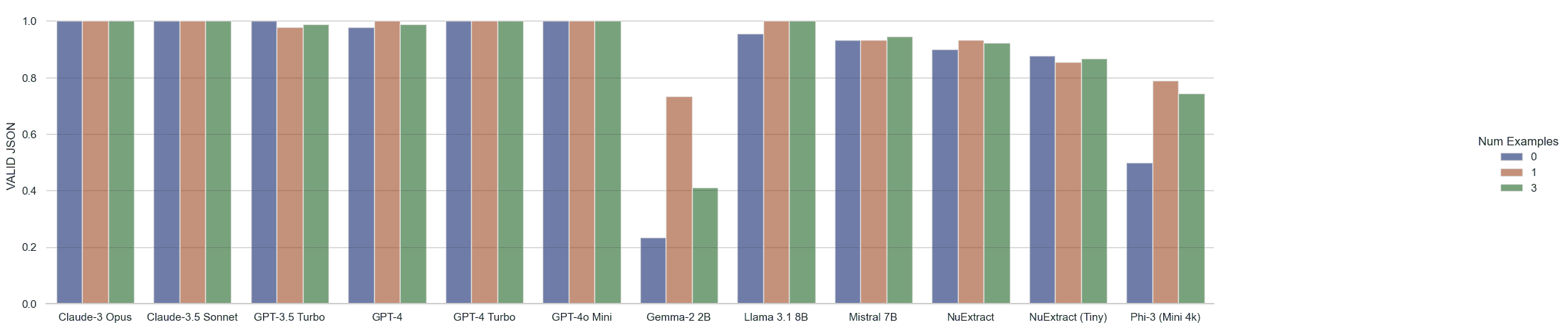
Even absent function calling or constraint decoding, Anthropic and OpenAI both prove quite capable of generating valid JSON. The most common failure case for GPT-3.5 was a relatively innocuous “running out of tokens”, with NuExtract falling prey to the same more often than not. We attempted to recover the partial JSON when a model wasn’t able to close a tag and moved forward with it when this was the case.

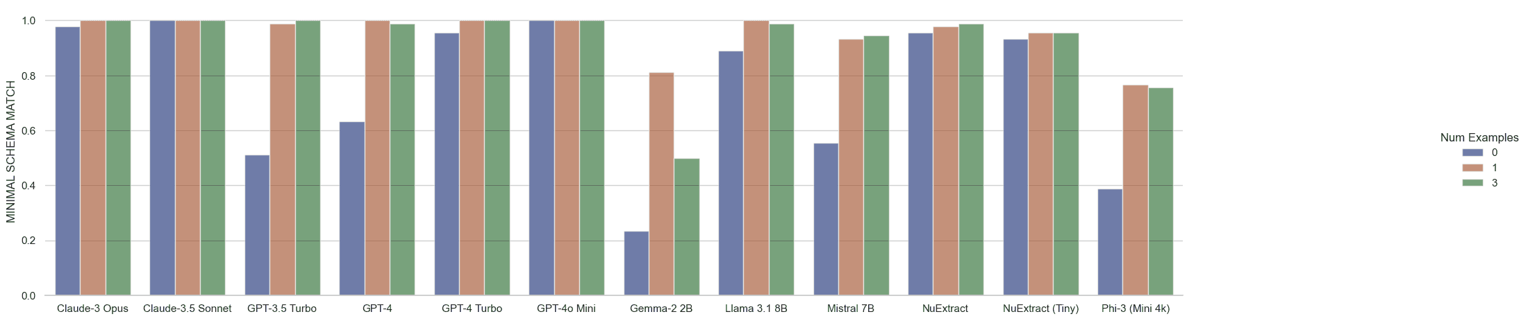
Moving on to focus on model outputs, we can notice an oddity in GPT-3.5 Turbo. The presence of a “properties” field in the JSON schema seems to have frequently hamstrung the model in the zero-shot case, leading it astray and causing it to add all child values inside a “properties”: {“foo”: …} sub-object instead of using the fields inside the properties as the actual keys. Neither GPT-4 nor Claude seemed to demonstrate this same behavior.

Our last and most rigorous structural check: can we directly parse the unmodified model output into an object according to the Pydantic schema?

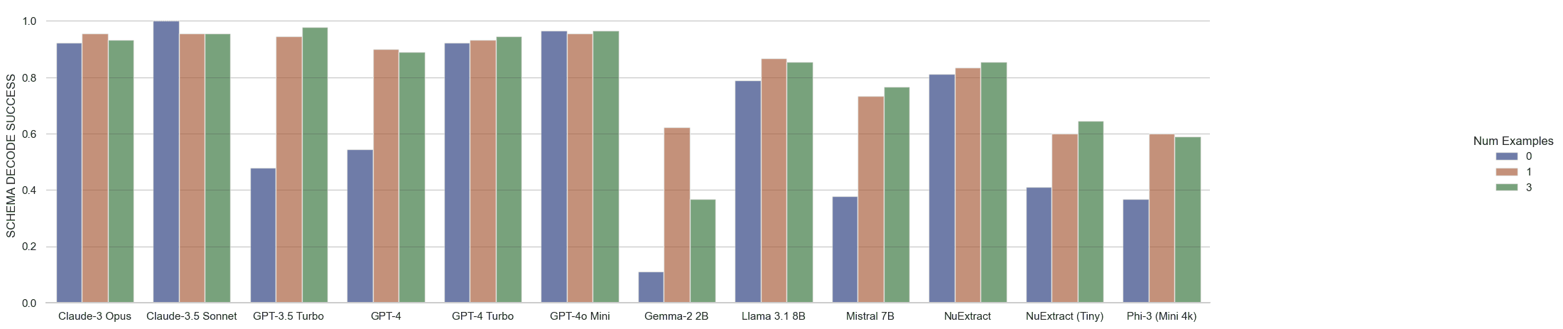
In addition to the standard and expected ‘valid JSON’ constraint, our decode enforces other constraints like range, non-null, etc. NuExtract-TINY here is at a particular disadvantage, as the format in which it has been trained to receive data does not specify type information or constraints, though it still manages to outperform the Phi-3 model on which it is based across the board.

Finally, we can look at our ‘eval score’, which is discussed in greater detail above. Once again, the primary takeaway from this diagram should not be the absolute performance of each model but performance of the models relative to each other. The y-axis has been rescaled in service of this goal.

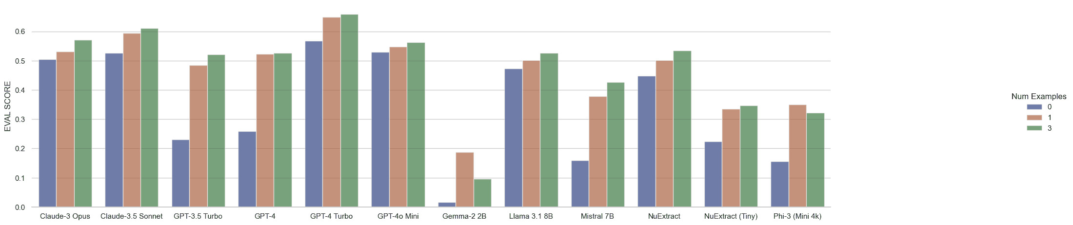
As one might expect, GPT-4-turbo is leading the pack with GPT-4o-mini, Claude-3 Sonnet, and Claude-3 Opus in close competition. There are two surprises in the data: first, both GPT-4 and GPT-3.5-turbo suffer in the zero-shot case from putting their outputs inside a “properties” field instead of using the properties mentioned in the output schema. Once an example is provided they recover to expected levels. The second surprise is how close NuExtract and Llama 3.1 are to the performance of GPT-4 and GPT-4o-Mini, even beating out GPT-3.5-turbo in some cases. Given that NuExtract is small enough to run comfortably on a 3090, this could be a compelling option.

JSON Mode (OpenAI) and Function calling.

By passing response_format={"type": "json_object"} into the OpenAI API client, one engages what Open AI calls “json mode”. This mode is automatically triggered when using function calling, but can be used separately. Relatedy, by passing a “tools” parameter, one can engage “Function Calling” mode. Function Calling is a simple phrase for a simple idea: give your large language model a description of the available ‘functions’ and the required parameters for each, then let the model decide.

Note that not all OpenAI models support json mode, and confusingly, some support function calling without supporting JSON mode.² Anthropic’s JSON mode, as of the time of writing, does not have a separate flag to engage JSON mode, but they do list JSON mode in their documentation.³

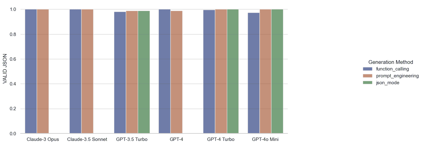
When it comes to ensuring valid JSON, neither function calling nor JSON mode give much in the way of benefits over prompt engineering. Nearly all generated JSON is well structured, with the few exceptions being due to truncations. The story changes when one tries to use Pydantic to directly interpret the JSON output of the models.

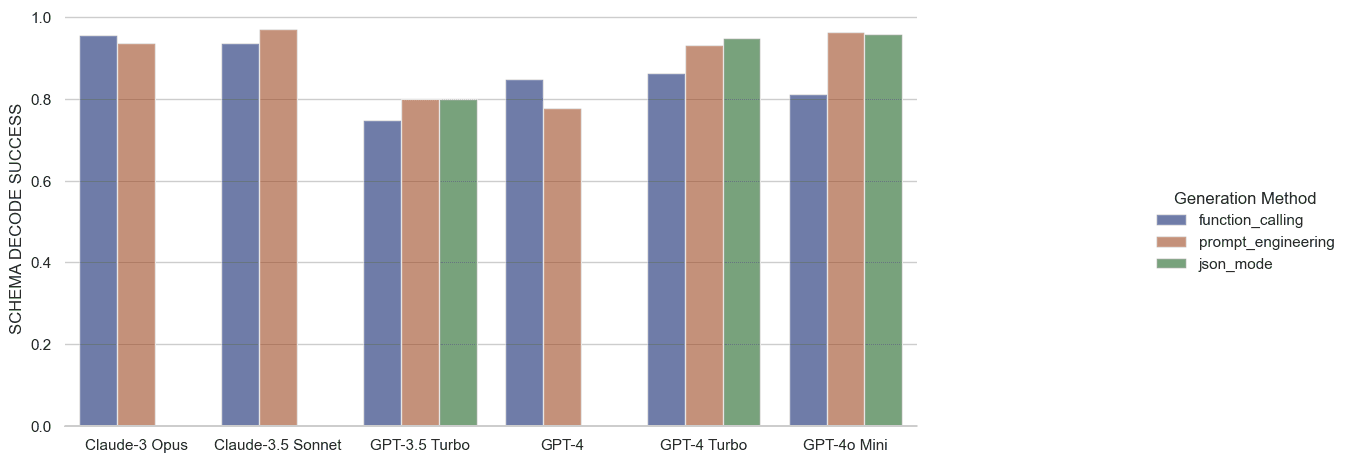
It may be surprising to see function calling falling short of prompt engineering and JSON mode in most cases, but this behavior seems to be consistent with observations in the Berkeley Function Calling Leaderboard.

The two most common failure cases for schema decoding were enum violations (i.e., passing in “human” when “person|place|thing” was a requirement) and number violations, like passing ‘null’ instead of 0 or a float 0.0 instead of 0. Missing fields were also a prominent contributor to decode failures, but again, those stemmed primarily from token limits. Moving on to quality:

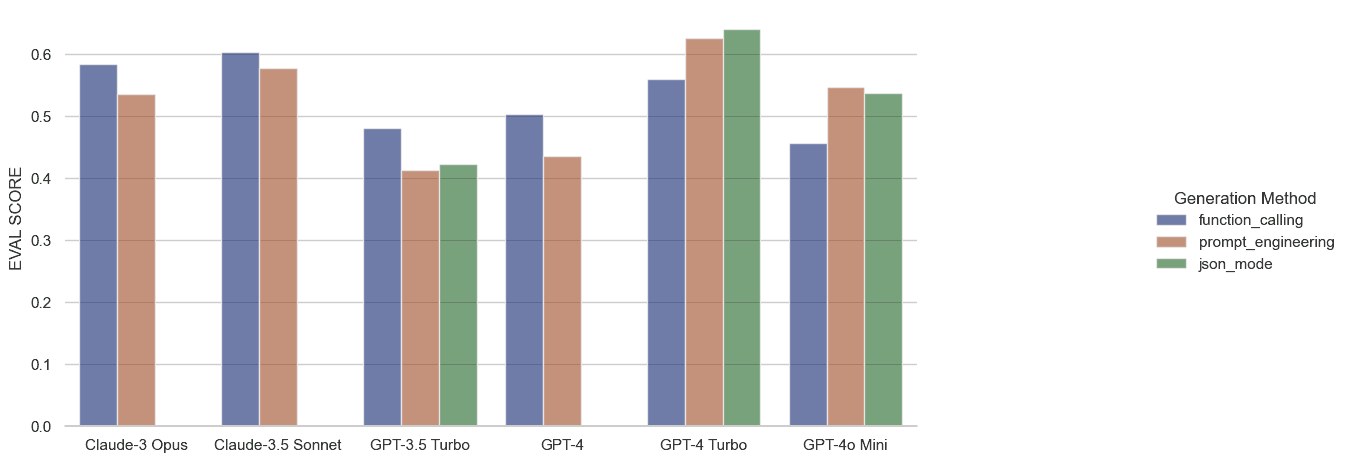
Anthropic and early versions of GPT seem to benefit from function calling, though only just. The cost overhead of tool use for Anthropic is measured in additional tokens, and if one assumes that their API calls will always result in a function call then the cost is on the order of 200 tokens/call.

Latency Considerations

Latency calculations include the round-trip time for a request to be filed from an open client connection. This does not include the time to negotiate a connection to host or resolve DNS, as these delays are highly variable and easy to negate by keeping a connection alive.

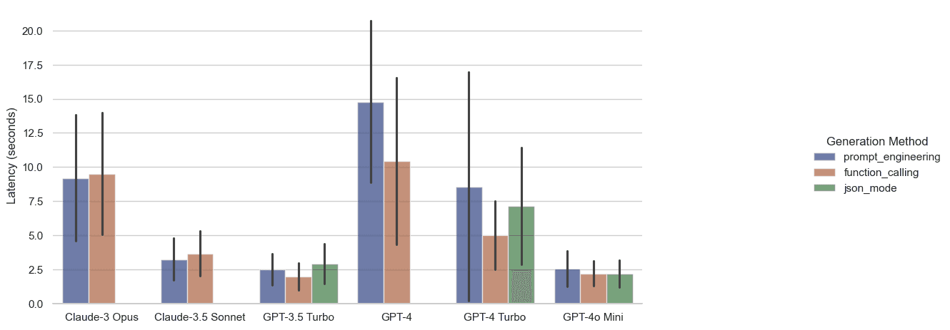
GPT-4o mini and GPT-3.5 Turbo are both strong contenders with the function calling mode providing even a slight latency improvement. Enabling JSON mode or Function Calling helps to stabilize the call time for GPT-4 Turbo, and Function Calling further reduces the latency over plain prompt engineering at a cost of additional input tokens.

Conclusions

GPT-4 Turbo remains the leader of the pack for structured data extraction, though at $5.00 per million input tokens and $15 per million output tokens, it’s also the most expensive and highest latency option. GPT-4o Mini has the is the budget alternative that also offers significantly lower latency than nearly all other options and a lower cost than GPT-4 Turbo. NuExtract and Llama 3.1 are both fairly remarkable self-hosted options and are highly comparable performance-wise, though self-hosting is not a panacea and latency numbers are very much a function of hosting provider, hardware, etc. Our overall recommendation is GPT-4o Mini for the combination of high quality output and low latency in processing. The added latency and 15x cost increase of GPT-4 Turbo makes it difficult to recommend over Mini for most use cases.

Footnotes

1. Please do not attempt to split an orange into its constituent particles without appropriate parental supervision. ↩

2. https://platform.openai.com/docs/guides/function-calling ↩

3. https://docs.anthropic.com/en/docs/build-with-claude/tool-use ↩